About to Data
I used Cyclistic’s “historical trip data” to analyze and identify trend
The location of the data can be found here:
https://divvy-tripdata.s3.amazonaws.com/index.html
Note: For the purposes of this case study, the datasets are appropriate and will enable the analyst to answer the business questions. The data has been made available by Motivate International Inc. under this license.
It should be noted that Cyclistic Bike-Share is a fictional company. The data has been cleansed of private onfo such as names, addresses, credit card info, etc prior Divvy Bikes posting the data online for use. You may see files with ‘Divvy’ in the names or code with Divvy present. This is just a formality as the files used have the true to lifes company name and branding.
Tools Used For This Case Study…
Microsoft Excel – I used Excel to initialially look at the data, do minor cleaning and preperation. I used Excel because I have more experience with it.
Microsoft SQL Server Management Studio – I used SSMS to do more data cleaning. I used SSMS to prepare the data for further queries and to build CSV files for import into Tableau. I used SSMS because I have a lot more experience with it. I knew I was going to use SQL more so I went with what I was comfortable with.
Tableau Public – I used Tableau for my data visualization. I did so for a couple reasons. Firstly, it was the system taught in the Google Data Anayst Pro course. Secondly, my current employer uses Tableau and I felt that it probably would be good to learn it a little more.
Microsoft Powerpoint – I used Powerpoint for my presentation.
Cleaning Process
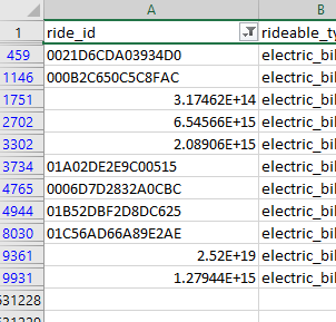
When I first downloaded and opened up the Divvy-Tripdata files a few things jumped out real quick. Firstly, I notice that ride_id column presented some row oddly. They would present as scientific notation.
This was because Excel made a few assumptions. It saw that these particular ride_id’s were either just numbers OR the only had an ‘E’ in them. I had to convert the ride_id column to string text. This solved that issue and I applied it to all the other files.
This prompted me to look further into the files and I started noticing that there were quite a few empty values in important areas of the data. Primarily things such as missing station data and the geo tracking data (latitude and longitude).
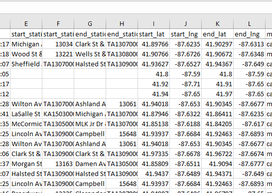
I knew from my initial thoughts on the data I wanted to include geo data in someway. I noticed that when a station name was missing it was also – in most cases – accompanied with less than precise geo data. I also knew the data size was far to large to work with so I determined that I would remove items to make a more suitable sample size. I could have removed the rows in Excel but decide to do that step with SQL in SSMS as it is better suited to handle larger data sets. These are the things I felt needed to be done in Excel. Due to the large data sets I felt that SQL was also better suited to combine all the data into one large set of data. I exported the data as a CSV (comma seperated value) file for import in SSMS as a flat file.
I took the 12 CSV files and imported them into SSMS as tables. At that time I did run into a few errors. SSMS will make a estimate of what type of data type. The data type it tried to assign threw errors and wouldnt import. So, I had to reassign the types from nvarchar(50) to varchar(MAX). Once the tables were created, I combined them into a single table.
I named it dbo.cyclistic_tripdata_2021-2022. This table included all the empty cells that were present in the excel files. But, now they were NULLs.

I also found a station that wasnt complete but had more complete data. This was a station witha station name ‘351’. Later I found a station that looked like a testing warehouse. It was the Divvy Warehouse (‘Hubbard Bike-checking (LBS-WH-TEST)’). I removed this later with a different script.
I removed the NULL rows and station ‘351’ in the initial creation of the ‘master’ tripdata table. During this time, I also added a column with ride length. I used the code below to query the Cyclistic Tripdata for Aug. 2021 to July 2022. This also alerted me to rides that were interestily small. Like rides only a minute or two. So, I ammended the script to cull out rides less than 5 minutes. My thought being that these rides may not be actual rides. Again thinking that maybe someone actually starts the process of renting a bike but does not complete it.
SELECT
	[ride_id],
	[rideable_type],
	[started_at],
	[ended_at],
	DATEADD(SECOND, DATEDIFF(SECOND, started_at, ended_at), CONVERT(time(0), '00:00')) AS ride_length,
	DATENAME(WEEKDAY, started_at) AS day_of_week, -- adds col for named day of the week
	DATENAME(MONTH, started_at) AS month_of_trip, -- adds col for named month
	[start_station_name],
	[start_station_id],
	[end_station_name],
	[end_station_id],
	[start_lat],
	[start_lng],
	[end_lat],
	[end_lng],
	[member_casual]
  FROM [dbo].[cyclistic_tripdata_2021_2022]
  WHERE ( -- this set will remove all rows with nulls.
	ride_id IS NOT NULL AND
	rideable_type IS NOT NULL AND
	started_at IS NOT NULL AND
	ended_at IS NOT NULL AND
	start_station_name IS NOT NULL AND
	start_station_id IS NOT NULL AND
	end_station_name  IS NOT NULL AND
	end_station_id  IS NOT NULL
	)
		AND
		DATEDIFF(MINUTE, started_at, ended_at) > 5 -- removes rides less than 5 minutes
		AND
		start_station_name != '351' -- removes the station 351 (unknown)
ORDER BY started_at
This script also adds 2 columns: one for day of the week and one for month. This query was then made into a new table to be used as a base for further queries later in the preperation phase.
Analysis Preparation
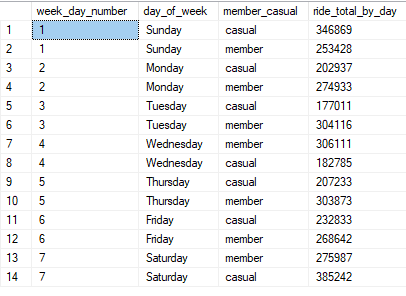
When originally looking at the data, I immediately saw a few things that I felt would be useful to use in my presentation. The first thing I wanted to add was a “Ride per day of the week” chart. I thought it would be nice to see if there was any difference between members and casual riders based on the day of the week. To do that, I wrote a script to count all the rides by member and casual, and sort by the day of the week.
SELECT
	DATEPART(WEEKDAY, started_at) AS week_day_number,
	day_of_week,
	member_casual,
	COUNT(*) AS ride_total_by_day
FROM dbo.cyclistic_tripdata_2021_2022
GROUP BY DATEPART(WEEKDAY, started_at), day_of_week, member_casual
ORDER BY DATEPART(WEEKDAY, started_at)
This resulted with the below results. You will see 4 rows. The first being week_day_number. This was so I could sort by the number. This info was visualized in the final presentation.
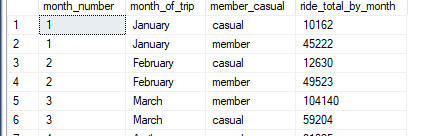
I then determined that a breakdown similar to the day of week would shed light on whether the month of year had any bering on ride totals. The code was quite similar to the above code.
SELECT
	DATEPART(MONTH, started_at) AS month_number,
	month_of_trip,
	member_casual,
	COUNT(*) AS ride_total_by_month
FROM dbo.cyclistic_tripdata_2021_2022
GROUP BY DATEPART(MONTH, started_at), month_of_trip, member_casual
ORDER BY DATEPART(MONTH, started_at)
This also resulted in similar look results, only with months rather than days.
Seeing this monthly ride information I noticed that there was also a noticable difference between members and casual riders in regards to how long they used the actual bikes. So I looked at rides within specific ranges. <15 mins, 15-30 mins, 30-45mins, 45-60mins, and >60. This actually shed a lot more light on things than I originally thought. The query for the 15-30 min range is below.
/* The #'s in the WHERE clause can be changed to make the query find different ranges. */
SELECT
	member_casual,
	COUNT(*) AS rides_between_15_and_30
FROM dbo.cyclistic_tripdata_2021_2022
WHERE (
	DATEDIFF(MINUTE, started_at, ended_at) >= 15 AND
	DATEDIFF(MINUTE, started_at, ended_at) < 29
	)
GROUP BY member_casual
This showed me the difference in how long members use the bike compared to how long casual riders use the bikes. While the example doesnt fully show it. The was quite a difference. And, it confirmed that there was a large difference in how the different users used the bikes. Especially when looking at longer rides. The longer the ride, the bigger the difference.

I then wondered whether there was preference in bike offerings between the members and casual customers.
SELECT
	rideable_type,
	member_casual,
	COUNT(*) AS type_ttl
FROM dbo.cyclistic_tripdata_2021_2022
GROUP BY rideable_type, member_casual
This actual shed a little more light on the differences between the members and casual riders. The one big difference being that in a whole year, a member did not use docked bikes.

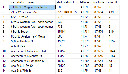
When I first saw the data (during the cleaning process) I really liked the geographical data (latitude and longitude). The main issue was the data was somewhat inaccurate. It wasnt that it was not trust worthy. It was that it was to trust worthy. By this I mean that it was incredibly accurate. So the biggest problem was that when someone rented a bike it would log the geo data….within feet. What that meant was that a rental done at a location such as Michigan Ave & Oak St may have many different latitudes and longitudes. This caused grouping and sorting issues. I had to devise a way to group the stations (so only one version of the station would show up in the query result) with a single latitude and longitude for that station. I had to do a lot of verification with google maps to confirm my results matched the actual location. I decided to average the geo data and also round it up to the 4th decimal place. I was able to confirm that the locations and the geo data somewhat matched up to their real life location. The following query is what I used to produce the result used in my presentation.
SELECT
	station_max.start_station_name,
	station_max.start_station_id,
	ROUND(AVG(station_max.start_lat),3) AS latitude,
	ROUND(AVG(station_max.start_lng),3) AS longitude,
	MAX(station_max.station_ttl) AS max_ttl
FROM (
	SELECT
		[start_station_name],
		[start_station_id],
		[start_lat],
		[start_lng],
		COUNT(start_station_name) AS station_ttl
	FROM [dbo].[cyclistic_tripdata_2021_2022]
	WHERE (start_station_id != 'Hubbard Bike-checking (LBS-WH-TEST)')
	GROUP BY
		[start_station_name],
		[start_station_id],
		[start_lat],
		[start_lng]
	) AS station_max
GROUP BY
	station_max.start_station_id,
	station_max.start_station_name
The result was a table that show each individual station, the station ID, the latitude, longitude, and the largest total of rides. The biggest issue with this particular table was that because of the differences between the rides geo data, I couldnt get both a sum of all the rides for a spedific station AND a latitude and longitude for the station. So I knew that I would need to pull data from another table when I moved onto the presentation part of the process. This query gave me all the info I need to plot a map.
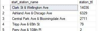
Knowing I needed a accurate total per station (as the geo data table would not produce an accurate count). I queried a simple total for each individual station.
SELECT
	start_station_name,
	COUNT(*)
FROM dbo.cyclistic_tripdata_2021_2022
GROUP BY start_station_name
This query resulted in a list of each station and a total for all rides from that station. This allowed me a way to also include the accurate total per station. This would also provide me a way to show what stations are the most popular and thusly able to determine whether the location may shed light on differences between members and casula customers.
At this point I determined I had enough data extracted to make some solid recommendations with some compelling visuals.
